SmollerTTS, a 2.81M-parameter English TTS model
SmollerTTS is a 2.81M-parameter English voice that runs on your browser’s CPU. The weights take up 11.34 MB. Try it below.
Starting small
I originally wanted a model under a million parameters that spoke several languages. The early versions sounded robotic and skipped words. I kept changing things, but it was hard to tell whether pronunciation, the acoustic model or the waveform decoder was responsible.
I narrowed it to one English speaker and a pretrained HiFi-GAN V2 vocoder. That made debugging easier. I could compare audio reconstructed from a real recording with audio made from my model’s predictions. The vocoder was the same in both, so the difference pointed back to the acoustic model.
The result is my own 1.88M-parameter acoustic network, trained from scratch on LJSpeech, paired with a 0.93M-parameter vocoder. Both run locally; your text stays on your device.
From text to a waveform
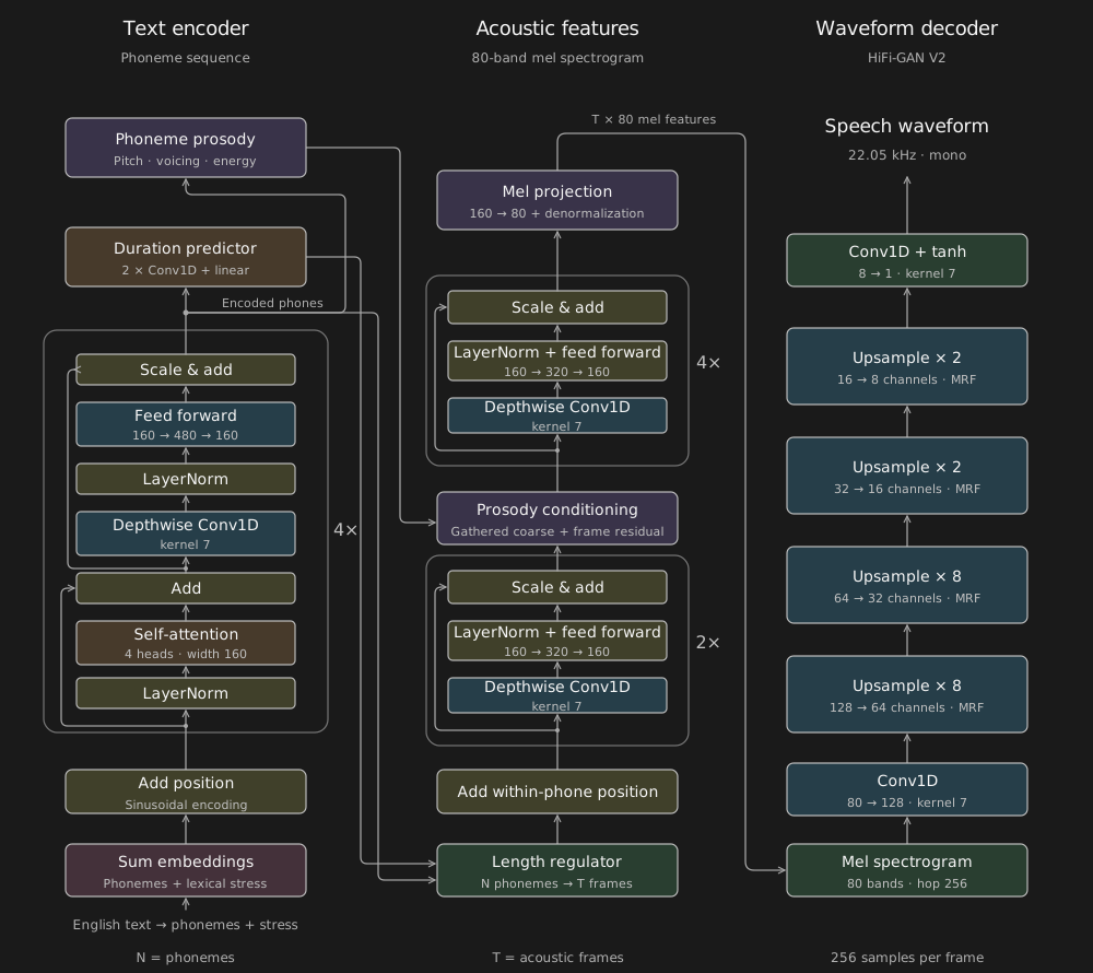
Text becomes phonemes, the model predicts their timing and acoustic features, and the vocoder turns those features into audio. Each chunk of speech is predicted in parallel.
View full architecture
Text and pronunciation
The frontend expands dates, times and money into words before converting them to phonemes. “$12.99” needs a spoken reading such as “twelve dollars and ninety-nine cents.” Stress markers tell the model which syllables should receive emphasis.
This was one place where an apparently simple fix backfired. Splitting difficult words into familiar pieces helped some examples but made ordinary words worse. The current frontend keeps dictionary pronunciations, only splits tested compounds automatically, and lets you supply an explicit pronunciation when needed.
Timing and acoustic features
Phoneme and stress embeddings are summed at a width of 160, with positional encoding added. Four encoder blocks combine four-head self-attention, depthwise convolutions and small feed-forward layers. Attention gives each phone context from the sentence; the convolutions capture local patterns.
A duration head predicts how many frames each phone should occupy. The length regulator repeats the N encoded phones in H by their predicted durations, giving T audio frames in total. A position signal within each phone lets its beginning and ending sound different.
Six convolutional frame blocks then predict an 80-band mel spectrogram, a compact description of how sound energy changes over time. Pitch, voicing and energy predictions condition this stage. The acoustic network contains 1,882,807 parameters.
Each frame block uses a depthwise convolution to mix nearby frames, followed by two linear layers that expand the features from 160 to 320 channels and bring them back to 160.
Here, X is the input frame sequence, LN is layer normalization, and W₁ and W₂ are learned linear layers including their biases. The learned channel-wise scale α controls how much the block adds to its input. Padding masks are omitted from the equation.
The waveform decoder
The frozen HiFi-GAN LJ_V2 generator converts those mel features into a 22,050 Hz mono waveform. Its four upsampling stages expand each frame by 8 × 8 × 2 × 2, or 256 audio samples. Residual branches with different receptive fields help model the waveform at several scales.
I use the published vocoder weights, which contribute 925,985 parameters. Its training discriminators are not needed for playback. Together, the acoustic model and vocoder total 2,808,792 parameters.
The acoustic model learns normalized mel features. Before sending its predictions to HiFi-GAN, I restore their original scale using statistics calculated from the training set.
M contains the log-mel features and Z their normalized values. The indices t and f identify a frame and mel band; μ and σ are the per-band training mean and standard deviation. Hats mark predictions, and x̂ is the generated waveform.
Training the acoustic model
I used LJSpeech, roughly 24 hours of recordings from one English speaker. The released run used 12,134 accepted training clips, about 22.12 hours, with separate development recordings and reserved test IDs. A single speaker kept the voice consistent without needing a speaker-conditioning system.
Forced alignment estimates where each phoneme occurs in the recordings, giving the model a duration target. WORLD extracts pitch and voicing. The preparation code computes energy and mel features, then calculates normalization statistics from training frames only.
The mel features have to match what the vocoder was trained to consume. That includes the magnitude convention, frequency range, window, hop, padding and log scale. Getting the tensor shape right is not enough. I also compare the exported graphs with the Python model to catch changes introduced on the way to the browser.
The acoustic model starts from random weights. The release recipe uses 10,000 updates with AdamW, complete utterances and a learning-rate warm-up. The loss combines mel reconstruction, changes between neighbouring mel frames, phoneme duration and prosody prediction. The frozen vocoder does not participate in this training loop.
Training settings
| Initialization | Random; seed 2718 |
|---|---|
| Batch | Up to 24 utterances; 12,000 padded frames |
| Optimizer | AdamW; β = (0.9, 0.98); weight decay 0.01 |
| Learning rate | 5 × 10⁻⁴ base; 300-step warm-up; 20,000-step half-life |
| Mel features | 80 bands; FFT 1024; hop 256; 0–8,000 Hz |
| Precision | FP32; TF32 enabled on CUDA |
The loss uses absolute error for mel reconstruction, frame-to-frame differences for the delta term, and squared error on log durations. Prosody combines pitch, energy and voicing. The full configuration is in the repository.
I still want to address a mismatch between training and inference. The decoder receives recorded prosody during training and predicted prosody when generating speech. Training it to cope with its own imperfect predictions is one of the next experiments I want to run.
Getting it into the browser
The model is exported as three FP32 ONNX graphs for the encoder, frame decoder and vocoder. JavaScript handles text processing and length regulation between them. A Web Worker runs inference on a single WebAssembly CPU thread, keeping the page responsive while audio is generated.
| Graph | File size | Job |
|---|---|---|
| Encoder | 5.00 MB | Phones, durations, coarse prosody |
| Frame decoder | 2.59 MB | Frame features and mel prediction |
| Vocoder | 3.74 MB | Mel features to waveform |
| Total weights | 11.34 MB | 2.81M parameters, FP32 |
Including the runtime and pronunciation files, the download is about 30 MB. The weights are FP32, with no quantization yet. I checked the exported model against the Python version to catch differences in the browser output.
The full demo plays longer text in chunks, starting as soon as the first is ready. This article’s player waits for the complete output. Repeated requests can reuse cached audio.
Speech quality vs. model size (rough)
I scored SmollerTTS on the four English prompts used by tts-bench and added it to their published results.
| Runtime | Source | ||||
|---|---|---|---|---|---|
| AuroraTTS-100K | 95.6K | 3.09 | 11.58% | Linux CPU |  |
| sanoTTS Amy | 1.46M | 3.82 | 6.69% | Linux CPU | |
| SmollerTTS | 2.81M | 3.55 | 6.69% | Browser CPU |  |
| Inflect-Nano v2 | 3.96M | 4.43 | 5.30% | Linux CPU | |
| tiny-voca | 4.50M | 4.40 | 6.57% | Linux CPU | |
| Vaniq-Edge | 8.91M | 4.27 | 9.34% | Linux CPU | |
| Inflect-Micro v2 | 9.36M | 4.44 | 3.03% | Linux CPU | |
| KittenTTS Nano 0.8 | 15.00M | 4.29 | 4.42% | Linux CPU | |
| Piper | 15.00M | 4.31 | 4.42% | Linux CPU | |
| SteerTTS (no refiner) | 23.10M | 3.95 | 6.49% | Linux CPU | |
| Underdog Woof | 38.20M | 4.45 | 8.96% | Linux CPU | |
| SteerTTS | 40.80M | 4.08 | 6.49% | Linux CPU | |
| LinnetTTS | 41.40M | 4.18 | 8.84% | Linux CPU | |
| SupraTTS 0.1 Beta | 43.50M | 3.30 | 5.81% | Linux CPU | |
| MeloTTS | 52.00M | 3.76 | 15.20% | Linux CPU | |
| ribt | 54.00M | 4.25 | 7.20% | Linux CPU | |
| Soprano 1.1 80M | 80.00M | 4.03 | 5.18% | Linux CPU | |
| Kokoro | 82.00M | 4.50 | 8.08% | Linux CPU | |
| Hojo-TTS-Light 40M | 84.50M | 4.36 | 11.87% | Linux CPU | |
| Supertonic 3 | 99.00M | 4.46 | 7.45% | Linux CPU | |
| MOSS-TTS-Nano | 100.00M | 4.10 | 5.93% | Linux CPU | |
| OpenVoice v2 | 100.00M | 4.10 | 13.73% | Linux CPU | |
| Pocket-TTS v4 | 100.00M | 4.33 | 5.30% | Linux CPU | |
| Sopro V2 Turbo | 120.00M | 4.00 | 8.01% | Linux CPU | |
| Sopro V2 Turbo (streaming) | 120.00M | 3.64 | 7.45% | Linux CPU | |
| LuxTTS | 123.00M | 2.30 | 61.10% | Linux CPU | |
| ZipVoice | 123.00M | 4.01 | 7.20% | Linux CPU | |
| Scylla's Band | 131.00M | 4.16 | 2.90% | Linux CPU | |
| StyleTTS 2 | 148.00M | 4.37 | 17.66% | Linux CPU | |
| Hojo-TTS-Light 80M | 167.00M | 4.34 | 6.69% | Linux CPU | |
| Audio8 TTS Preview 0.1B | 170.00M | 4.40 | 11.33% | Linux CPU | |
| NeuTTS Nano | 229.00M | 4.12 | 27.27% | Linux CPU | |
| F5-TTS v1 | 330.00M | 4.02 | 21.41% | Linux CPU | |
| Magpie-TTS | 357.00M | 4.38 | 7.95% | Linux CPU | |
| CosyVoice 3 0.5B | 500.00M | 3.97 | 5.93% | Linux CUDA | |
| Fish Speech 1.5 | 500.00M | 3.87 | 16.46% | Linux CPU | |
| MiraTTS | 500.00M | 3.80 | 9.98% | Linux CUDA | |
| VibeVoice Realtime 0.5B | 500.00M | 4.22 | 10.10% | Linux CPU | |
| Qwen3-TTS 0.6B CustomVoice | 600.00M | 4.37 | 8.71% | Linux CPU | |
| Audio8 TTS 0.6B (compiled) | 601.00M | 4.43 | 5.81% | Linux CUDA | |
| Audio8 TTS Preview 0.6B | 601.00M | 4.43 | 8.71% | Linux CPU | |
| Audio8 TTS Realistic 0.6B | 601.00M | 4.51 | 2.90% | Linux CPU | |
| ChatterBox Turbo | 744.00M | 4.26 | 7.45% | Linux CPU | |
| NeuTTS Air | 748.00M | 3.79 | 13.89% | Linux CPU | |
| Coqui XTTS-v2 | 750.00M | 4.19 | 11.27% | Linux CPU | |
| ZONOS3-Mini (ggml Q4) | 800.00M | 3.93 | 8.08% | Linux CPU | |
| Parler-TTS Mini v1 | 878.00M | 3.55 | 15.33% | Linux CPU | |
| IndexTTS-2.5 | 970.00M | 3.77 | 15.32% | Linux CPU | |
| OmniVoice | 1.00B | 4.27 | 4.29% | Linux CPU | |
| OuteTTS 1.0 1B | 1.00B | 4.43 | 8.59% | Linux CUDA | |
| Sesame CSM-1B | 1.00B | 4.19 | 19.18% | Linux CPU | |
| ChatterBox | 1.20B | 4.44 | 5.05% | Linux CPU | |
| Mars5-TTS | 1.20B | 3.53 | 34.13% | Linux CUDA | |
| MetaVoice-1B | 1.20B | 3.80 | 33.73% | Linux CUDA | |
| LongCat-AudioDiT 1B | 1.42B | 4.05 | 9.34% | Linux CUDA | |
| Ming-3.0-TTS 0.5B | 1.48B | 4.04 | 7.32% | Linux CUDA | |
| IndexTTS-2 | 1.50B | 3.75 | 9.47% | Linux CPU | |
| LFM2.5-Audio 1.5B | 1.50B | 4.37 | 9.47% | Linux CPU | |
| VibeVoice 1.5B | 1.50B | 3.71 | 16.81% | Linux CPU | |
| AuK | 1.53B | 4.16 | 6.31% | Linux CUDA | |
| AuK-Flash | 1.53B | 4.27 | 5.68% | Linux CUDA | |
| Dia 1.6B-0626 | 1.60B | 3.03 | 10.15% | Linux CUDA | |
| Zonos v0.1 | 1.60B | 4.10 | 7.45% | Linux CPU | |
| KittenTTS 2 | 1.70B | 4.51 | 14.14% | Linux CPU | |
| KittenTTS 2 (C++ CPU) | 1.70B | 4.51 | 5.81% | Linux CPU | |
| Qwen3-TTS 1.7B (CUDA-graph) | 1.70B | 4.30 | 13.42% | Linux CUDA | |
| Qwen3-TTS 1.7B Base | 1.70B | 4.11 | 8.08% | Linux CPU | |
| dots.tts (soar) | 2.00B | 3.65 | 7.32% | Linux CUDA | |
| LFM3-Audio 2B | 2.00B | 4.44 | 3.66% | Linux CPU | |
| VoxCPM2 | 2.00B | 4.03 | 4.29% | Linux CPU | |
| FireRedTTS3 | 2.12B | 4.13 | 10.23% | Linux CUDA | |
| Echo-TTS | 2.80B | 4.21 | 7.45% | Linux CUDA | |
| Maya1 | 3.00B | 4.47 | 5.05% | Linux CUDA | |
| Orpheus TTS | 3.00B | 4.00 | 10.23% | Linux CUDA | |
| Step-Audio-EditX | 3.00B | 4.23 | 10.14% | Linux CUDA | |
| DramaBox | 3.30B | 4.23 | 9.34% | Linux CUDA | |
| LongCat-AudioDiT 3.5B | 3.83B | 4.34 | 7.95% | Linux CUDA | |
| Fish Speech S2-Pro | 4.00B | 4.31 | 8.84% | Linux CUDA | |
| Higgs Audio v3 TTS | 4.00B | 4.48 | 8.08% | Linux CUDA | |
| VibeVoice 7B | 7.00B | 3.50 | 8.37% | Linux CUDA | |
| MOSS-TTS v1.0 | 8.00B | 4.22 | 7.18% | Linux CUDA | |
| MOSS-TTS v1.5 | 8.00B | 4.22 | 8.08% | Linux CUDA | |
| Miso TTS 8B | 8.20B | 4.07 | 39.66% | Linux CUDA | |
| Ming-3.0-TTS tiny | 8.98B | 4.36 | 5.18% | Linux CUDA | |
| Fish Audio Drama 3 (ComfyUI port) | 35.90B | 4.46 | 5.05% | Linux CUDA | |
SmollerTTS scores 3.55 UTMOS and 6.69% mean prompt WER here. The WER uses Whisper large-v3. Different voices, runtimes and some evaluator revisions make this a rough overview, and four sentences cannot establish a reliable ranking.
A closer comparison with tiny-voca
I also rendered a separate set of 48 prompts with SmollerTTS and two tiny-voca voices. The set covers everyday speech, narration, dialogue, numbers, technical terms and longer passages. All three voices completed every prompt.
| Model / voice | Parameters | UTMOS | WER |
|---|---|---|---|
| SmollerTTS / LJ | 2.81M | 3.77 | 0.92% |
| tiny-voca F2 | 4.54M | 4.43 | 0.26% |
| tiny-voca M2 | 4.54M | 4.33 | 0.39% |
This test uses Whisper small.en and corpus-level WER, so it should be read separately from the graph. I normalized time and unit formatting for all models after inspecting the transcripts; SmollerTTS scored 1.71% WER before that change. The full results include the details.
SmollerTTS is smaller, but tiny-voca scores better on both metrics. That matches what I hear. The words are often clear, but the delivery can still sound flat. A low word error rate does not mean a voice is pleasant to listen to.
What I would improve next
Timing and prosody come first. Longer training runs and bigger decoders did not consistently help in the early experiments. I want to test changes against fixed prompts, with people listening as well as automated scores. After that, I would like to try quantization to reduce the download.
Try it, or help to hillclimb it
The demo, source and weights are public. The repository includes data preparation, training, checkpoint resume, listening tools and ONNX export.
The training guide documents how to train from random initialization. It reproduces the released architecture and recipe, but the complete accepted-recording list from the original run has not been recovered, so it does not promise identical training data selection or checkpoint bytes.
If you’re interested in helping out, send me an email, open a pull request, or file an issue in the repository.
References
Keith Ito and Linda Johnson. The LJ Speech Dataset. 2017.
Jungil Kong, Jaehyeon Kim and Jaekyoung Bae. HiFi-GAN: Generative Adversarial Networks for Efficient and High Fidelity Speech Synthesis. NeurIPS, 2020. Code and pretrained weights.
Takaaki Saeki, Detai Xin, Wataru Nakata, Tomoki Koriyama, Shinnosuke Takamichi and Hiroshi Saruwatari. UTMOS: UTokyo-SaruLab System for VoiceMOS Challenge 2022. Interspeech, 2022. Implementation.
5uck1ess and contributors. tts-bench. Benchmark snapshot
1dd3a81, accessed 19 November 2026.
Cite this post
@misc{chan2026smollertts,
  title = {{SmollerTTS}, a 2.81M-parameter English text-to-speech model},
  author = {Chan, Dun Li},
  year = {2026},
  month = {nov},
  howpublished = {\url{https://dunlichan.com/writings/smollertts/}},
  note = {Blog post}
}